Pre-processing

Quality Control

Remove Empty Droplet using drokick

adata

AnnData object with n_obs × n_vars = 9000 × 33538
    obs: 'type', 'sample', 'batch'
    var: 'gene_ids', 'feature_types', 'genome'

#@title Dropkick run
# To skip running this code cell run the following command

%%script echo skipping



# simple preprocessing of anndata object to get metrics for plot
adata = dk.recipe_dropkick(adata, n_hvgs=None, X_final="raw_counts")

skipping

print(adata)

print("===================================================\n")

# print(adata_empty)

AnnData object with n_obs × n_vars = 9000 × 33538
    obs: 'type', 'sample', 'batch'
    var: 'gene_ids', 'feature_types', 'genome'
===================================================

%%script echo skipping


qc_plt = dk.qc_summary(adata)

skipping

We can see from the total counts profile (top) that this sample has relatively low background (“empty” droplets), as indicated by the steep dropoff in counts and genes around barcode 5,000.

The dropout rate distribution also looks pretty good, with a steep increase in dropout rate following the first few highly-expressed genes (MALAT1, RPS27, B2M)

This tool preprocesses the data to automatically calculate thresholds on global metrics, then trains a glmnet-style logistic regression model to determine scores and labels for each barcode in the dataset describing likelihood of being a real cell (rather than empty droplet). The dropkick model is returned (adata_model), and contains scikit-learn-style attributes for further exploration. Scores and metrics are also added to the original AnnData object as part of the dk.dropkick function.

The n_jobs parameter will parallelize the model training. Since the default is 5-fold cross-validation, we’ll use 5 cores to quickly train dropkick.

%%script echo skipping


%time adata_model = dk.dropkick(adata, n_jobs=1)

skipping

Running dropkick interactively adds the following attributes to the input AnnData object:

• .obs[‘dropkick_score’] Probability of being a real cell Values closer to 0 indicate empty droplets with high ambient RNA content

• .obs[‘dropkick_label’] Binary label generated by using cutoff of 0.5 on ‘dropkick_score’ Dropkick’s best estimate of a “good” dataset User is encouraged to adjust the cutoff according to whether they are more concerned with false negatives or false positives

• .obs[] Metrics used for thresholding (metrics parameter, default [‘arcsinh_n_genes_by_counts’], are kept

%%script echo skipping

print(adata.obs['dropkick_score'])

print("=================================================")

print(adata.obs['dropkick_label'])

skipping

The score_plot function displays these barcodes in a scatter plot of ambient percentage (as calculated in the qc_summary plot above) versus total genes detected for each cell. The automated thresholds on the latter heuristic are overlayed to show the initial training labels given to the dropkick model.

%%script echo skipping


score_plt = dk.score_plot(adata)

skipping

%%script echo skipping


dk.coef_inventory(adata)

skipping

%%script echo skipping


coef_plt = dk.coef_plot(adata)

skipping

%%script echo skipping


print("Before empty drop removal :", adata.shape)

print("======================================================")

# make a copy of our AnnData object as adata_nonempty , keeping all barcodes kept by dropkick
adata = adata[(adata.obs.dropkick_label=="True"), :].copy()

print("After empty drop removal :", adata.shape)

skipping

adata

AnnData object with n_obs × n_vars = 9000 × 33538
    obs: 'type', 'sample', 'batch'
    var: 'gene_ids', 'feature_types', 'genome'

Calculate QC

Steps :

• Filter Zero count cells / cell with low number of detected genes

• Correction of Ambient RNA

• Doublet Detection

• Normalization (Pearson Residual transformation)

• Feature selection

• Dimensionality reduction

Note : In order to delete low quality cells , we have to jointly considered following qc metrices (so we don’t remove much cells) :

• Count Depth (if low means small or dying cell)

• Few genes per cell (dying cell)

• High mitochondrial genes fraction per cell (Mitochondria leaked
  out and cell ruptured)

Solution : using MAD (median absolute deviations) automatic method

         Mark cell oulier >  MAD >= 5 threshold

#@title Calculate QC Metrics 

# First Calculate QC Metrices for [ mt, ribo, hb ] and Counts related metrices

###==================================###########

# We calculate QC metrices for Mitochondrial fraction , ribosomal fraction and haemoglobin fraction
# And we have count related metrcies like Depth count (Total count) , n_genes_by_counts  , pct_counts_mt

# We use MAD (Median Deviation) of these metrices with threshold like nmads = 3 and represent cells as outlier 
# Then we use these ouliers cells to remove So we achieve filtering

###==================================###########



# mitochondrial genes
adata.var["mt"] = adata.var_names.str.startswith("MT-")
# ribosomal genes
adata.var["ribo"] = adata.var_names.str.startswith(("RPS", "RPL"))
# hemoglobin genes.
adata.var["hb"] = adata.var_names.str.contains(("^HB[^(P)]"))

adata.var.head()

	gene_ids	feature_types	genome	mt	ribo	hb
MIR1302-2HG	ENSG00000243485	Gene Expression	GRCh38	False	False	False
FAM138A	ENSG00000237613	Gene Expression	GRCh38	False	False	False
OR4F5	ENSG00000186092	Gene Expression	GRCh38	False	False	False
AL627309.1	ENSG00000238009	Gene Expression	GRCh38	False	False	False
AL627309.3	ENSG00000239945	Gene Expression	GRCh38	False	False	False

adata

AnnData object with n_obs × n_vars = 9000 × 33538
    obs: 'type', 'sample', 'batch'
    var: 'gene_ids', 'feature_types', 'genome', 'mt', 'ribo', 'hb'

sc.pp.calculate_qc_metrics(
    adata, qc_vars=["mt", "ribo", "hb"], inplace=True, percent_top=[20], log1p=False
)
adata

AnnData object with n_obs × n_vars = 9000 × 33538
    obs: 'type', 'sample', 'batch', 'n_genes_by_counts', 'total_counts', 'pct_counts_in_top_20_genes', 'total_counts_mt', 'pct_counts_mt', 'total_counts_ribo', 'pct_counts_ribo', 'total_counts_hb', 'pct_counts_hb'
    var: 'gene_ids', 'feature_types', 'genome', 'mt', 'ribo', 'hb', 'n_cells_by_counts', 'mean_counts', 'pct_dropout_by_counts', 'total_counts'

• n_genes_by_counts in .obs is the number of genes with positive counts in a cell,

• total_counts is the total number of counts for a cell, this might also be known as library size, and

• pct_counts_mt is the proportion of total counts for a cell which are mitochondrial.

adata.obs.head(3)

	type	sample	batch	n_genes_by_counts	total_counts	pct_counts_in_top_20_genes	total_counts_mt	pct_counts_mt	total_counts_ribo	pct_counts_ribo	total_counts_hb	pct_counts_hb
AGGGTCCCATGACCCG-1-0	Covid	covid_1	0	2140	7698.0	24.123149	525.0	6.819953	2564.0	33.307353	2.0	0.025981
TACCCACAGCGGGTTA-1-0	Covid	covid_1	0	3391	13416.0	21.414729	952.0	7.096005	2264.0	16.875373	6.0	0.044723
CCCAACTTCATATGGC-1-0	Covid	covid_1	0	3654	16498.0	22.402715	1253.0	7.594860	2723.0	16.505031	1.0	0.006061

Plot QC

Now we can Plot these calculated metrices . each dot represents cell in plot . Group by sample , so we can see for each sample how merics behaves

sc.pl.violin(adata, ['total_counts', 'n_genes_by_counts',  'pct_counts_mt','pct_counts_ribo', 'pct_counts_hb'],
             jitter=0.4, groupby = 'sample', rotation= 45)

As you can see, there is quite some difference in quality for the 4 datasets, with for instance the covid_15 sample having fewer cells with many detected genes and more mitochondrial content. As the ribosomal proteins are highly expressed they will make up a larger proportion of the transcriptional landscape when fewer of the lowly expressed genes are detected. And we can plot the different QC-measures as scatter plots.

sc.pl.violin(adata, ['total_counts', 'n_genes_by_counts',  'pct_counts_mt','pct_counts_ribo', 'pct_counts_hb'],
             jitter=0.4, groupby = 'type', rotation= 45)

sc.pl.scatter(adata, "total_counts", "n_genes_by_counts", color="pct_counts_mt", show= False,   legend_loc= "best")

<Axes: title={'center': 'pct counts mt'}, xlabel='total_counts', ylabel='n_genes_by_counts'>

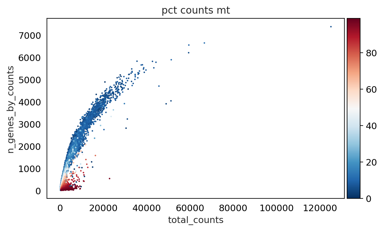
As we can see from above plot : genes with low counts have more percentage mitochondria and some cells have less mitochondria .

Filtering (Joint Effect)

We have to filter cells by considering joint effects by these WC metrics we have calculated in previous cells .

We use Automatic method MAD : which depends on Median and Standard deviation

We first calculate outliers by each od these QC effects

Filter Using Automatic Method : MAD

#@title Create outlier function  

# function that takes a metric, i.e. a column in .obs and the number of MADs (nmad)

# Function take 3 Arguments : 1) Adata object , 2) Metric colum for condition 3) nmads = 3 or 5 or ...?

def is_outlier(adata, metric: str, nmads: int):
    M = adata.obs[metric]
    outlier = (M < np.median(M) - nmads * median_abs_deviation(M)) | (
        np.median(M) + nmads * median_abs_deviation(M) < M
    )
    return outlier

adata.obs.head(3)

	type	sample	batch	n_genes_by_counts	total_counts	pct_counts_in_top_20_genes	total_counts_mt	pct_counts_mt	total_counts_ribo	pct_counts_ribo	total_counts_hb	pct_counts_hb
AGGGTCCCATGACCCG-1-0	Covid	covid_1	0	2140	7698.0	24.123149	525.0	6.819953	2564.0	33.307353	2.0	0.025981
TACCCACAGCGGGTTA-1-0	Covid	covid_1	0	3391	13416.0	21.414729	952.0	7.096005	2264.0	16.875373	6.0	0.044723
CCCAACTTCATATGGC-1-0	Covid	covid_1	0	3654	16498.0	22.402715	1253.0	7.594860	2723.0	16.505031	1.0	0.006061

#@title use QC metrices to find outlier cells 

adata.obs["outlier"] = (
    is_outlier(adata, "total_counts", 5)
    | is_outlier(adata, "n_genes_by_counts", 5)
    | is_outlier(adata, "pct_counts_in_top_20_genes", 5)
)


print(adata.obs.outlier.value_counts())

adata.obs.head(3)

False    6898
True     2102
Name: outlier, dtype: int64

	type	sample	batch	n_genes_by_counts	total_counts	pct_counts_in_top_20_genes	total_counts_mt	pct_counts_mt	total_counts_ribo	pct_counts_ribo	total_counts_hb	pct_counts_hb	outlier
AGGGTCCCATGACCCG-1-0	Covid	covid_1	0	2140	7698.0	24.123149	525.0	6.819953	2564.0	33.307353	2.0	0.025981	False
TACCCACAGCGGGTTA-1-0	Covid	covid_1	0	3391	13416.0	21.414729	952.0	7.096005	2264.0	16.875373	6.0	0.044723	False
CCCAACTTCATATGGC-1-0	Covid	covid_1	0	3654	16498.0	22.402715	1253.0	7.594860	2723.0	16.505031	1.0	0.006061	False

#@title use Mitochondrial QC metric to find outlier cells

adata.obs["mt_outlier"] = is_outlier(adata, "pct_counts_mt", 3) | (
    adata.obs["pct_counts_mt"] > 8    #cells with a percentage of mitochondrial counts exceeding 8 % are filtered out
)

print(adata.obs.mt_outlier.value_counts())

adata.obs.head(3)

False    4762
True     4238
Name: mt_outlier, dtype: int64

	type	sample	batch	n_genes_by_counts	total_counts	pct_counts_in_top_20_genes	total_counts_mt	pct_counts_mt	total_counts_ribo	pct_counts_ribo	total_counts_hb	pct_counts_hb	outlier	mt_outlier
AGGGTCCCATGACCCG-1-0	Covid	covid_1	0	2140	7698.0	24.123149	525.0	6.819953	2564.0	33.307353	2.0	0.025981	False	False
TACCCACAGCGGGTTA-1-0	Covid	covid_1	0	3391	13416.0	21.414729	952.0	7.096005	2264.0	16.875373	6.0	0.044723	False	False
CCCAACTTCATATGGC-1-0	Covid	covid_1	0	3654	16498.0	22.402715	1253.0	7.594860	2723.0	16.505031	1.0	0.006061	False	False

#@title Filter out cells with Above QC metrices :

print(f"Total number of cells  Before Filtering : {adata.n_obs}")
adata = adata[(~adata.obs.outlier) & (~adata.obs.mt_outlier)].copy()

print("")

print(f"Number of cells after filtering of low quality cells: {adata.n_obs}")

Total number of cells  Before Filtering : 9000

Number of cells after filtering of low quality cells: 4205

Plot Filtered QC

#@title Filtered Data Plot

sc.pl.violin(adata, ['total_counts', 'n_genes_by_counts',  'pct_counts_mt','pct_counts_ribo', 'pct_counts_hb'],
             jitter=0.4, groupby = 'sample', rotation= 45)

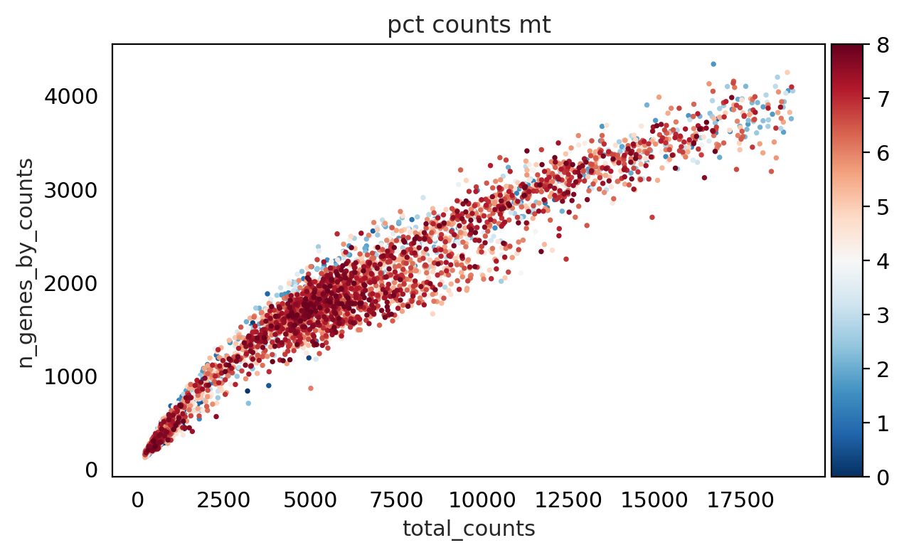
sc.pl.scatter(adata, "total_counts", "n_genes_by_counts", color="pct_counts_mt", show= False,   legend_loc= "best")

<Axes: title={'center': 'pct counts mt'}, xlabel='total_counts', ylabel='n_genes_by_counts'>

ambient RNA correction using scAR :

To work with scAR we need following :

• raw Anndata (unfitered from sequencing machine , which contain Empty droplets and cells with only free mRNA )

• Filtered data

Then we estimate Ambient profile from raw and filtered data

Then we use Machine learning to train data to identify Ambient RNA and then we correct count matrix with respect to Ambient profile

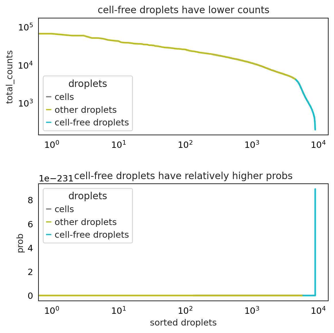
setup_anndata is inspired by EmptyDrops which assumes that cell-free droplets are sampled from a multinomial distribution.

1. It first calculates an initial ambient profile by averaging all droplets in raw_adata

2. It tested whether droplets fit the multinomial distribution (the ambient profile as the prob parameter). The relatively high probabilities suggest cell-free droplets

3. It re-calculates the ambient profile using the identified cell-free droplets

4. It repeats step 2 and step 3 for iterations

5. The final ambient profile is saved in adata.uns

#@title Read adata_raw

adata_raw = sc.read_h5ad("/content/drive/MyDrive/scRNA_using_Python/Objects/adata_raw_covid.h5ad")

adata_raw

AnnData object with n_obs × n_vars = 9000 × 33538
    obs: 'type', 'sample', 'batch'
    var: 'gene_ids', 'feature_types', 'genome'

#@title Estimate the ambient profile



setup_anndata(
    adata = adata,
    raw_adata = adata_raw,
    prob = 0.895,
    kneeplot = True
)

2023-05-28 05:45:56|INFO|setup_anndata|Randomly sample 9000 droplets from 9000 droplets.
INFO:setup_anndata:Randomly sample 9000 droplets from 9000 droplets.
2023-05-28 05:45:56|INFO|setup_anndata|Estimating ambient profile for ['Gene Expression']
Categories (1, object): ['Gene Expression']...
INFO:setup_anndata:Estimating ambient profile for ['Gene Expression']
Categories (1, object): ['Gene Expression']...
2023-05-28 05:46:04|INFO|setup_anndata|Iteration: 1
INFO:setup_anndata:Iteration: 1
2023-05-28 05:46:12|INFO|setup_anndata|Iteration: 2
INFO:setup_anndata:Iteration: 2
2023-05-28 05:46:20|INFO|setup_anndata|Iteration: 3
INFO:setup_anndata:Iteration: 3
2023-05-28 05:46:20|INFO|setup_anndata|Estimated ambient profile for Gene Expression saved in adata.uns
INFO:setup_anndata:Estimated ambient profile for Gene Expression saved in adata.uns
2023-05-28 05:46:20|INFO|setup_anndata|Estimated ambient profile for all features saved in adata.uns
INFO:setup_anndata:Estimated ambient profile for all features saved in adata.uns

#@title Traine Ambient Data 

adata_scar = model(raw_count=adata, # In the case of Anndata object, scar will automatically use the estimated ambient_profile present in adata.uns.
                      ambient_profile=adata.uns['ambient_profile_Gene Expression'],
                      feature_type='mRNA',
                      sparsity=1,
                      device='cuda' # Both cpu and cuda are supported.
                     )

adata_scar.train(epochs=200,
                    batch_size=64,
                    verbose=True
                   )

# After training, we can infer the native true signal
adata_scar.inference(batch_size=256)  # by defaut, batch_size = None, set a batch_size if getting a memory issue

2023-05-28 05:46:42|INFO|model|cuda will be used.
INFO:model:cuda will be used.
2023-05-28 05:46:46|INFO|VAE|Running VAE using the following param set:
INFO:VAE:Running VAE using the following param set:
2023-05-28 05:46:46|INFO|VAE|...denoised count type: mRNA
INFO:VAE:...denoised count type: mRNA
2023-05-28 05:46:46|INFO|VAE|...count model: binomial
INFO:VAE:...count model: binomial
2023-05-28 05:46:46|INFO|VAE|...num_input_feature: 33538
INFO:VAE:...num_input_feature: 33538
2023-05-28 05:46:46|INFO|VAE|...NN_layer1: 150
INFO:VAE:...NN_layer1: 150
2023-05-28 05:46:46|INFO|VAE|...NN_layer2: 100
INFO:VAE:...NN_layer2: 100
2023-05-28 05:46:46|INFO|VAE|...latent_space: 15
INFO:VAE:...latent_space: 15
2023-05-28 05:46:46|INFO|VAE|...dropout_prob: 0.00
INFO:VAE:...dropout_prob: 0.00
2023-05-28 05:46:46|INFO|VAE|...expected data sparsity: 1.00
INFO:VAE:...expected data sparsity: 1.00
2023-05-28 05:46:46|INFO|model|kld_weight: 1.00e-05
INFO:model:kld_weight: 1.00e-05
2023-05-28 05:46:46|INFO|model|learning rate: 1.00e-03
INFO:model:learning rate: 1.00e-03
2023-05-28 05:46:46|INFO|model|lr_step_size: 5
INFO:model:lr_step_size: 5
2023-05-28 05:46:46|INFO|model|lr_gamma: 0.97
INFO:model:lr_gamma: 0.97

Training: 100%|██████████| 200/200 [03:38<00:00,  1.09s/it, Loss=5.4521e+03]

#@title Denoised counts :
denoised_count = pd.DataFrame(adata_scar.native_counts, index=adata.obs_names, columns=adata.var_names)

print("")
print(denoised_count.shape)
print("=================================================")
denoised_count.head()

(4205, 33538)
=================================================

	MIR1302-2HG	FAM138A	OR4F5	AL627309.1	AL627309.3	AL627309.2	AL627309.4	AL732372.1	OR4F29	AC114498.1	...	AC007325.2	BX072566.1	AL354822.1	AC023491.2	AC004556.1	AC233755.2	AC233755.1	AC240274.1	AC213203.1	FAM231C
AGGGTCCCATGACCCG-1-0	0.0	0.0	0.0	0.0	0.0	0.0	0.0	0.0	0.0	0.0	...	0.0	0.0	0.0	0.0	0.0	0.0	0.0	0.0	0.0	0.0
TACCCACAGCGGGTTA-1-0	0.0	0.0	0.0	0.0	0.0	0.0	0.0	0.0	0.0	0.0	...	0.0	0.0	0.0	0.0	0.0	0.0	0.0	0.0	0.0	0.0
CCCAACTTCATATGGC-1-0	0.0	0.0	0.0	0.0	0.0	0.0	0.0	0.0	0.0	0.0	...	0.0	0.0	0.0	0.0	0.0	0.0	0.0	0.0	0.0	0.0
ATTCCTAGTGACTGTT-1-0	0.0	0.0	0.0	0.0	0.0	0.0	0.0	0.0	0.0	0.0	...	0.0	0.0	0.0	0.0	0.0	0.0	0.0	0.0	0.0	0.0
CCTAAGACAGATTAAG-1-0	0.0	0.0	0.0	0.0	0.0	0.0	0.0	0.0	0.0	0.0	...	0.0	0.0	0.0	0.0	0.0	0.0	0.0	0.0	0.0	0.0

5 rows × 33538 columns

#@title Add Denoised count (Ambient RNA corrected ) to adata :

adata

adata.layers["counts"] = adata.X
adata.layers["ambient_counts"] = adata_scar.native_counts
adata.X = adata.layers["ambient_counts"]


adata

AnnData object with n_obs × n_vars = 4205 × 33538
    obs: 'type', 'sample', 'batch', 'n_genes_by_counts', 'total_counts', 'pct_counts_in_top_20_genes', 'total_counts_mt', 'pct_counts_mt', 'total_counts_ribo', 'pct_counts_ribo', 'total_counts_hb', 'pct_counts_hb', 'outlier', 'mt_outlier'
    var: 'gene_ids', 'feature_types', 'genome', 'mt', 'ribo', 'hb', 'n_cells_by_counts', 'mean_counts', 'pct_dropout_by_counts', 'total_counts'
    uns: 'sample_colors', 'type_colors', 'ambient_profile_Gene Expression', 'ambient_profile_all'
    layers: 'counts', 'ambient_counts'

adata.var.head()

	gene_ids	feature_types	genome	mt	ribo	hb	n_cells_by_counts	mean_counts	pct_dropout_by_counts	total_counts
MIR1302-2HG	ENSG00000243485	Gene Expression	GRCh38	False	False	False	0	0.000000	100.000000	0.0
FAM138A	ENSG00000237613	Gene Expression	GRCh38	False	False	False	0	0.000000	100.000000	0.0
OR4F5	ENSG00000186092	Gene Expression	GRCh38	False	False	False	0	0.000000	100.000000	0.0
AL627309.1	ENSG00000238009	Gene Expression	GRCh38	False	False	False	25	0.002778	99.722222	25.0
AL627309.3	ENSG00000239945	Gene Expression	GRCh38	False	False	False	1	0.000111	99.988889	1.0

Filter Genes

#@title Filter genes :
print(f"Total number of genes: {adata.n_vars}")

# Min 20 cells - filters out 0 count genes
sc.pp.filter_genes(adata, min_cells=20)
print(f"Number of genes after cell filter: {adata.n_vars}")

Total number of genes: 33538
Number of genes after cell filter: 7662

# As we have . we can remove genes correspond to Mirochondria , Ribosomal and MALAT1
# Because High level of MALAT1 and MT referes to Technical variation

 # group genes with MALAT1 , MT and HB and remove 
malat1 = adata.var_names.str.startswith('MALAT1')
mito_genes = adata.var_names.str.startswith('MT-')
hb_genes = adata.var_names.str.contains('^HB[^(P)]')

remove = np.add(mito_genes, malat1)
remove = np.add(remove, hb_genes)
keep = np.invert(remove)

print("before removal of genes :" , adata.n_obs, adata.n_vars)

adata = adata[:,keep]

print("After removal of genes :" ,adata.n_obs, adata.n_vars)

before removal of genes : 4205 7662
After removal of genes : 4205 7650

#@title install pybiomart

Cell Cycle Scoring

#@title Cell Cycle scoring : 


!if [ ! -f data/regev_lab_cell_cycle_genes.txt ]; then curl -o data/regev_lab_cell_cycle_genes.txt https://raw.githubusercontent.com/theislab/scanpy_usage/master/180209_cell_cycle/data/regev_lab_cell_cycle_genes.txt; fi

cell_cycle_genes = [x.strip() for x in open('./data/regev_lab_cell_cycle_genes.txt')]
print(len(cell_cycle_genes))

# Split into 2 lists
s_genes = cell_cycle_genes[:43]
g2m_genes = cell_cycle_genes[43:]

cell_cycle_genes = [x for x in cell_cycle_genes if x in adata.var_names]
print(len(cell_cycle_genes))

97
33

# save normalized counts in raw slot.
adata.cycle = adata

# normalize to depth 10 000
sc.pp.normalize_per_cell(adata.cycle, counts_per_cell_after=1e4)

# logaritmize
sc.pp.log1p(adata.cycle)

# scale
sc.pp.scale(adata.cycle)

sc.tl.score_genes_cell_cycle(adata.cycle, s_genes=s_genes, g2m_genes=g2m_genes)

adata.cycle.obs.phase.value_counts()

G1     1474
G2M    1371
S      1360
Name: phase, dtype: int64

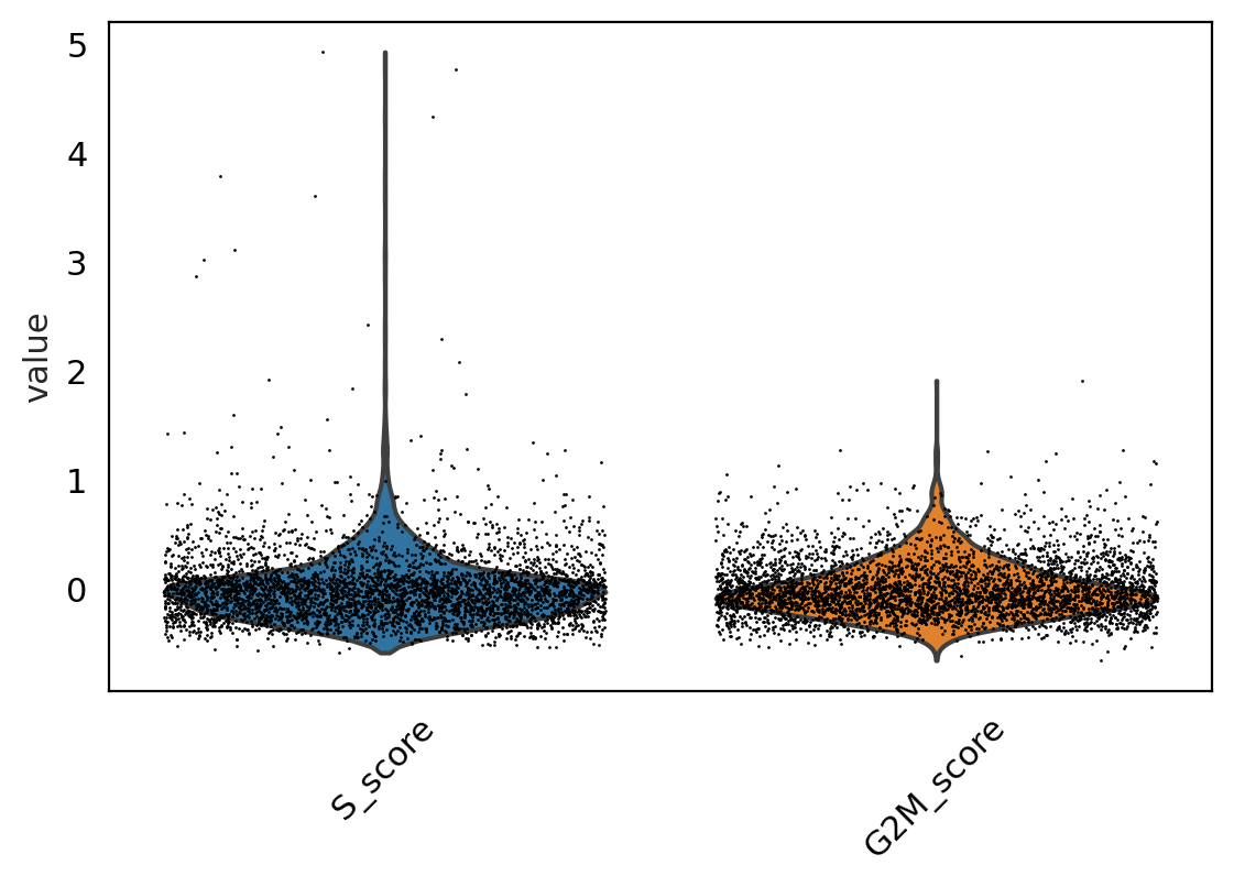
sc.pl.violin(adata.cycle, ['S_score', 'G2M_score'],
             jitter=0.4,  rotation=45)

Doublet detection

#@title Doublet Detection :

print(adata.shape)

(4205, 7650)

# Change the layer of count  to Ambient counts 

adata.X = adata.layers["ambient_counts"]

#@title Run scvi setup model

scvi.model.SCVI.setup_anndata(adata)
vae = scvi.model.SCVI(adata)
vae.train()

INFO:pytorch_lightning.utilities.rank_zero:GPU available: True (cuda), used: True
INFO:pytorch_lightning.utilities.rank_zero:TPU available: False, using: 0 TPU cores
INFO:pytorch_lightning.utilities.rank_zero:IPU available: False, using: 0 IPUs
INFO:pytorch_lightning.utilities.rank_zero:HPU available: False, using: 0 HPUs
INFO:pytorch_lightning.accelerators.cuda:LOCAL_RANK: 0 - CUDA_VISIBLE_DEVICES: [0]

Epoch 400/400: 100%|██████████| 400/400 [02:27<00:00,  2.70it/s, loss=3.52e+03, v_num=1]

INFO:pytorch_lightning.utilities.rank_zero:`Trainer.fit` stopped: `max_epochs=400` reached.

Epoch 400/400: 100%|██████████| 400/400 [02:27<00:00,  2.71it/s, loss=3.52e+03, v_num=1]

#@title Train solo model 

solo = scvi.external.SOLO.from_scvi_model(vae)
solo.train()

INFO     Creating doublets, preparing SOLO model.                                                                  

INFO:pytorch_lightning.utilities.rank_zero:GPU available: True (cuda), used: True
INFO:pytorch_lightning.utilities.rank_zero:TPU available: False, using: 0 TPU cores
INFO:pytorch_lightning.utilities.rank_zero:IPU available: False, using: 0 IPUs
INFO:pytorch_lightning.utilities.rank_zero:HPU available: False, using: 0 HPUs
INFO:pytorch_lightning.accelerators.cuda:LOCAL_RANK: 0 - CUDA_VISIBLE_DEVICES: [0]

Epoch 400/400: 100%|██████████| 400/400 [02:03<00:00,  3.24it/s, loss=0.339, v_num=1]

INFO:pytorch_lightning.utilities.rank_zero:`Trainer.fit` stopped: `max_epochs=400` reached.

Epoch 400/400: 100%|██████████| 400/400 [02:03<00:00,  3.23it/s, loss=0.339, v_num=1]

#@title Predict the Doublet

df = solo.predict()
df['prediction'] = solo.predict(soft = False)
df.index = df.index.map(lambda x: x[:-2])

df

	doublet	singlet	prediction
AGGGTCCCATGACCCG-1-0	-1.240547	1.317724	singlet
TACCCACAGCGGGTTA-1-0	0.230032	-0.015135	doublet
CCCAACTTCATATGGC-1-0	0.087104	0.086796	doublet
ATTCCTAGTGACTGTT-1-0	-1.723657	1.353531	singlet
CCTAAGACAGATTAAG-1-0	-1.451537	1.859437	singlet
...	...	...	...
GCTGCAGTCTGTCAGA-14-5	-1.007731	0.915832	singlet
GAGGCCTTCTCCTGCA-14-5	-0.019297	0.247610	singlet
CCCTAACAGTTTCTTC-14-5	-0.336324	-0.266451	singlet
GGGATGATCAAGCTTG-14-5	0.087399	-0.348760	doublet
CAATGACCACTGCATA-14-5	0.385331	-0.194242	doublet

4205 rows × 3 columns

#@title Number of Doublets:

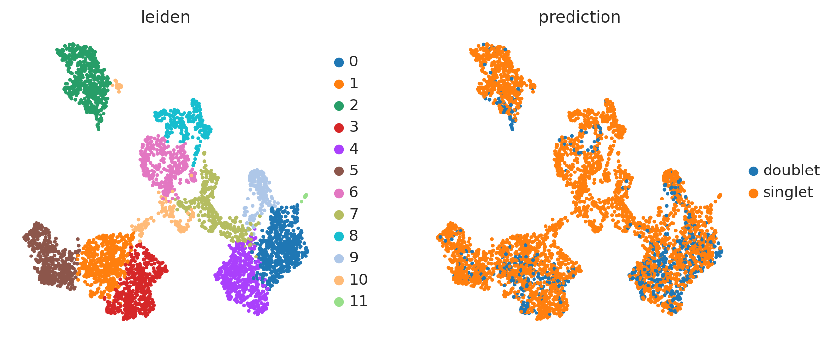
len(df[df.prediction == 'doublet'])  # pretty high number

669

#THIS STEP IS NOT NECESSARY, just to visuallize results
adata_doublet = adata

adata_doublet

AnnData object with n_obs × n_vars = 4205 × 7650
    obs: 'type', 'sample', 'batch', 'n_genes_by_counts', 'total_counts', 'pct_counts_in_top_20_genes', 'total_counts_mt', 'pct_counts_mt', 'total_counts_ribo', 'pct_counts_ribo', 'total_counts_hb', 'pct_counts_hb', 'outlier', 'mt_outlier', 'n_counts', 'S_score', 'G2M_score', 'phase', '_scvi_batch', '_scvi_labels'
    var: 'gene_ids', 'feature_types', 'genome', 'mt', 'ribo', 'hb', 'n_cells_by_counts', 'mean_counts', 'pct_dropout_by_counts', 'total_counts', 'n_cells', 'mean', 'std'
    uns: 'sample_colors', 'type_colors', 'ambient_profile_Gene Expression', 'ambient_profile_all', 'log1p', '_scvi_uuid', '_scvi_manager_uuid'
    layers: 'counts', 'ambient_counts'

adata_doublet.obs['prediction'] = df.prediction
sc.pp.normalize_total(adata_doublet, target_sum = 1e4)
sc.pp.log1p(adata_doublet)
sc.tl.pca(adata_doublet)
sc.pp.neighbors(adata_doublet)
sc.tl.umap(adata_doublet)
sc.tl.leiden(adata_doublet, resolution = 0.5)

with rc_context({'figure.figsize': (4, 4)}):
    sc.pl.umap(adata_doublet, color = ['leiden', 'prediction'])

doublet_d = dict(zip(df.index, df.prediction))

def doublet_function(x):
    try:
        return doublet_d[x]
    except:
        return 'filtered'

adata.obs['doublet'] = adata.obs.index.map(doublet_function)

adata

AnnData object with n_obs × n_vars = 4205 × 7650
    obs: 'type', 'sample', 'batch', 'n_genes_by_counts', 'total_counts', 'pct_counts_in_top_20_genes', 'total_counts_mt', 'pct_counts_mt', 'total_counts_ribo', 'pct_counts_ribo', 'total_counts_hb', 'pct_counts_hb', 'outlier', 'mt_outlier', 'n_counts', 'S_score', 'G2M_score', 'phase', '_scvi_batch', '_scvi_labels', 'prediction', 'leiden', 'doublet'
    var: 'gene_ids', 'feature_types', 'genome', 'mt', 'ribo', 'hb', 'n_cells_by_counts', 'mean_counts', 'pct_dropout_by_counts', 'total_counts', 'n_cells', 'mean', 'std'
    uns: 'sample_colors', 'type_colors', 'ambient_profile_Gene Expression', 'ambient_profile_all', 'log1p', '_scvi_uuid', '_scvi_manager_uuid', 'pca', 'neighbors', 'umap', 'leiden', 'leiden_colors', 'prediction_colors'
    obsm: 'X_pca', 'X_umap'
    varm: 'PCs'
    layers: 'counts', 'ambient_counts'
    obsp: 'distances', 'connectivities'

#@title remove predicted doublets

adata = adata[adata.obs.doublet == 'singlet']

adata

View of AnnData object with n_obs × n_vars = 3536 × 7650
    obs: 'type', 'sample', 'batch', 'n_genes_by_counts', 'total_counts', 'pct_counts_in_top_20_genes', 'total_counts_mt', 'pct_counts_mt', 'total_counts_ribo', 'pct_counts_ribo', 'total_counts_hb', 'pct_counts_hb', 'outlier', 'mt_outlier', 'n_counts', 'S_score', 'G2M_score', 'phase', '_scvi_batch', '_scvi_labels', 'prediction', 'leiden', 'doublet'
    var: 'gene_ids', 'feature_types', 'genome', 'mt', 'ribo', 'hb', 'n_cells_by_counts', 'mean_counts', 'pct_dropout_by_counts', 'total_counts', 'n_cells', 'mean', 'std'
    uns: 'sample_colors', 'type_colors', 'ambient_profile_Gene Expression', 'ambient_profile_all', 'log1p', '_scvi_uuid', '_scvi_manager_uuid', 'pca', 'neighbors', 'umap', 'leiden', 'leiden_colors', 'prediction_colors'
    obsm: 'X_pca', 'X_umap'
    varm: 'PCs'
    layers: 'counts', 'ambient_counts'
    obsp: 'distances', 'connectivities'

Save QC Filtered Data

save_file = 'Objects/sc_qc_filtered_covid.h5ad'
adata.write_h5ad(save_file)